Marketplace Supply Coverage: How to Find Hidden Gaps

What Marketplace Supply Coverage Reveals Before You Scale Demand

A marketplace with 50,000 listings can still fail to match buyers. Not because supply is missing. Because 80% of those listings sit in two categories, and the segments where buyers are searching are structurally empty.

This is the supply coverage problem. It looks like a product problem. It reads the attribution data as an acquisition-quality issue. Operators diagnose it as poor onboarding or bad targeting. The actual cause is simpler and harder to fix mid-scale: supply was never distributed where demand would land.

Supply coverage in a marketplace is the distribution of listings across the category, geography, and price segments where demand actually lands.

A marketplace with adequate aggregate supply but poor coverage leaves entire buyer segments unable to transact. Not because supply is missing. Because it is in the wrong place.

This article introduces the Supply Coverage Map: a three-axis diagnostic grid that makes structural gaps visible before demand acquisition begins. It connects measuring the liquidity threshold in a marketplace to match rate performance. The Supply Coverage Map answers the question that those two frameworks leave open: where specifically does supply need to go before you scale?

What Operators Get Wrong About Marketplace Supply

Most marketplace operators track supply count. Listings added per week, supply growth rate by quarter, and total inventory by category. These metrics feel like health signals.

They are not.

Aggregate supply is a volume metric. Coverage is a usability metric.

Aggregate supply count tells you how much supply exists. It does not tell you where that supply is relative to where demand is landing. A healthy aggregate number masks concentration in the segments that were easiest to fill and absence in the segments buyers are actually searching.

The pattern is predictable. Early supply acquisition follows the path of least resistance. Listings concentrate in the categories and markets where sellers are already active. Adjacent segments stay thin or empty. The aggregate count grows. The coverage distribution does not improve.

Operators discover this problem six months into a scaled demand acquisition program. Churn climbs. CAC rises. The data reads as targeting failure or product friction. The actual failure happened earlier: supply was never in the right place.

The table below shows how this plays out. The pre-scale signal is visible and measurable before spending begins. The post-scale symptom is the same problem made expensive.

Pre-Scale Signal	Post-Scale Symptom
Coverage gaps visible in specific intersections	CAC inflation across the entire program
Thin Coverage Ratios in target segments	Elevated segment-level churn after acquisition
Category or metro imbalance in listing distribution	False product friction diagnosis obscuring the real cause

Running the Supply Coverage Diagnostic before scale converts these symptoms into actionable signals before the acquisition budget is committed.

What Is Supply Coverage in a Marketplace?

Supply coverage is the distribution of supply inventory across the specific intersections where demand actually arrives. The measurement unit is the Coverage Ratio.

Coverage Ratio = Active Listings in Segment ÷ Estimated Demand Volume in Segment

Each intersection in your supply grid receives a Coverage Ratio. That ratio maps to one of three states:

Coverage Ratio Range	State	Interpretation
0.8 to 1.2+	Adequate	Demand arriving in this intersection can be served
0.3 to 0.79	Thin	Demand encounters friction; elevated churn risk
0 to 0.29	Gap	No viable supply; demand cannot transact

Structural gaps are not corrected by adding supply elsewhere in the marketplace.

If Industrial listings in Metro B have a Coverage Ratio of 0.04, adding more Office listings in Metro A does not help the Industrial buyer. The segments are not substitutes. The gap is structural because it lives in a specific intersection that demand cannot cross.

This is the diagnostic failure most operators make: treating aggregate supply count as a proxy for supply health, when supply health is a function of Coverage Ratios across specific intersections. Supply coverage determines whether a segment can reach the liquidity threshold in a marketplace at all. Without it, liquidity modeling operates on incomplete inputs.

The Supply Coverage Map Framework

The Supply Coverage Map is the segment-level precursor to liquidity threshold modeling. It answers the question liquidity measurement assumes: that supply exists in the right places. Without a coverage diagnostic, liquidity thresholds are calculated against a supply distribution that may be structurally misaligned with where demand will land.

The Supply Coverage Map maps supply inventory against demand across three axes: category, geography, and price or size segment. Each intersection receives a Coverage Ratio score and maps to a state: Adequate, Thin, or Gap.

Gap clusters — adjacent cells where multiple intersections score as Thin or Gap — identify where supply investment must go before demand acquisition scales. The output is not a list of problems. It is a ranked investment map. Gap clusters with high-demand signals receive investment first. Isolated gaps in low-demand segments get deferred.

Platform Revolution (Parker, Van Alstyne, and Choudary) identifies supply-demand balance as a core platform health variable. Their framework implies that aggregate counts can mask segment-level imbalances. The Supply Coverage Map makes that implication executable.

How Do You Diagnose Supply Gaps Before Scaling?

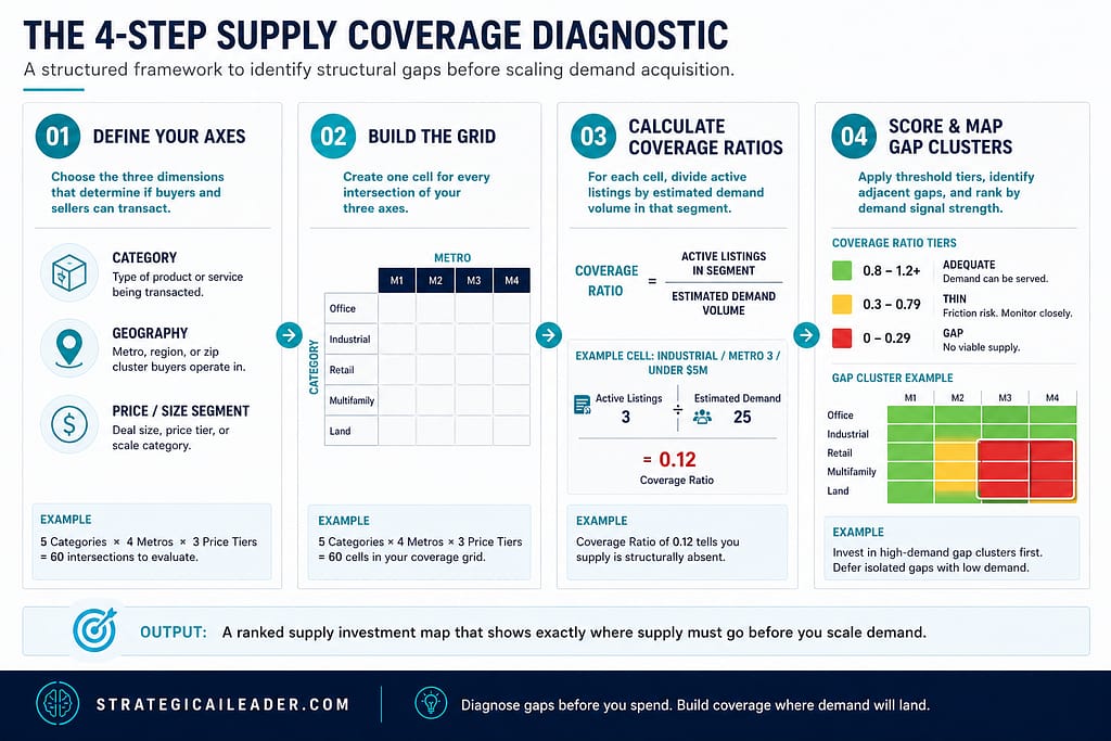
Running a Supply Gap Analysis using the Supply Coverage Map takes four steps.

Step 1: Define your axes. For most marketplaces: Category (type of product or service), Geography (metro, region, or zip cluster), and Price or Size Segment (deal size, price tier, or scale category). The right axes are the dimensions that determine whether a buyer and seller can transact. If buyers filter by these dimensions before contacting supply, those are your axes.

Step 2: Build the grid. Create one cell for every intersection of those three axes. A marketplace with 5 categories x4 metros x3 price tiers produces 60 cells. Grid size is determined by your market structure, not by what is convenient to measure.

Step 3: Calculate Coverage Ratios. For each cell, divide the number of active listings by the estimated demand volume. Demand signals can come from search queries, listing views, inquiry volume, or failed transaction attempts. A Coverage Ratio of 0.12 tells you something specific. “Supply looks healthy” tells you nothing.

Step 4: Score each cell and map gap clusters. Apply the threshold tiers: Adequate, Thin, or Gap. Identify where multiple adjacent cells score Thin or Gap. These are your gap clusters. Rank them by demand signal strength. The highest-demand gap clusters are your priority zones for supply investment.

I ran this diagnostic at MyEListing for the first time and expected to find a few thin segments. What came back was structural concentration, not isolated gaps.

What Happens Without Coverage Data

Before walking through the MyEListing case, it’s worth naming the generic failure pattern. It repeats across marketplace categories and deal types.

A marketplace launches a paid acquisition campaign targeting Metro 3 Industrial properties under $5M. The platform has 400 active listings overall. The aggregate looks healthy. Nobody specifically checks the Coverage Ratio for Metro 3 Industrial under $ 5M.

That Coverage Ratio is 0.12.

Demand arrives. Buyers search Metro 3 Industrial. They find two listings. Neither matches the deal size. Both are stale. They leave.

The match rate in that segment collapses. Churn climbs among buyers acquired in that campaign. CAC doubles by month two. The operations review reads: “acquisition targeting issue” or “onboarding drop-off.” The team optimizes ad creative and revises the onboarding flow.

Neither action addresses the real cause. There was no supply. The Coverage Ratio told that story before the campaign launched. Nobody looked.

This is why the coverage diagnostic runs before the acquisition program, not after.

What the Audit Revealed: The MyEListing Case

MyEListing is a commercial real estate marketplace connecting property owners, investors, and tenants. Commercial real estate is inherently segmented by hard filters. Property type, metro market, and deal size determine whether a buyer and a seller can transact. An Industrial buyer looking for a 50,000 sq ft facility in a secondary market cannot substitute an Office listing in a primary market. These filters are non-negotiable.

When we ran the Supply Coverage Map, the listing concentration became visible immediately. The majority of listings were concentrated in a small number of property types in a small number of primary markets. Adjacent property types, particularly Industrial and specialized retail formats, had thin Coverage Ratios in primary markets and structural gaps in secondary and tertiary metros. These were the same segments where demand acquisition was expected to land.

Investor Match Rate, the platform’s primary proxy for match quality, was lowest precisely in the gap segments. Buyers were arriving through demand acquisition programs, searching in uncovered intersections, and leaving without transacting. The attribution data appeared to be product friction or targeting noise. The actual problem was supply geography.

After supply investment was redirected toward the gap segments identified by the coverage map — rather than toward the already-covered segments where adding supply was easiest — Investor Match Rate improved 28%. That improvement did not come from better ad targeting or product changes. It came from fixing the right problem: supplying existing where demand was arriving.

That outcome changed how I think about the sequencing of supply and demand investment. The question is never “do we have enough supply?” It is “Does supply exist where demand will land?”

Supply coverage determines whether the match rate can rise at all. Without it, match rate improvements are bounded by structural gaps in supply distribution that targeting and product work cannot fix.

What Causes Supply Coverage Gaps in Two-Sided Platforms?

Supply coverage gaps form for predictable reasons.

Listing Concentration Risk is the most common pattern. Early supply acquisition follows ease rather than coverage logic. Listings are easiest to acquire where supply already exists. The platform develops a dense core and an empty periphery. Aggregate supply counts grow. Coverage Ratios in peripheral segments do not improve. The platform looks healthy by volume until demand acquisition starts landing in the empty periphery.

Cold-start segment inheritance is the second pattern. Categories that achieved adequate Coverage Ratios at initial market entry continue to receive investment. Categories that never reached coverage thresholds during early growth remain thin indefinitely. The early coverage distribution becomes the permanent coverage distribution unless a diagnostic explicitly identifies and targets the gaps.

The NFX Network Effects Library documents how early supply distribution decisions compound over time in two-sided markets. An underserved segment at the supply acquisition stage becomes a structural gap at the demand acquisition scale. The diagnostic needs to run before scale, not after, because fixing gaps post-scale requires reversing investment decisions already embedded in the platform’s supplier relationships.

Harvard Business Review’s work on two-sided platform competition identifies segment-level supply distribution as a competitive moat variable. Platforms that achieve adequate Coverage Ratios in segments where competitors have gaps create durable switching costs for both supply and demand. Segment-level coverage advantages compound into defensible liquidity zones that competitors cannot enter without rebuilding supplier relationships from scratch. The Supply Coverage Map makes that competitive positioning visible and actionable rather than intuitive.

When Should a Marketplace Operator Run a Supply Coverage Diagnostic?

Run the Supply Coverage Diagnostic before any significant demand acquisition investment. Specifically, run it when:

• You are preparing to scale ad spend or demand acquisition programs
• You are expanding into a new category or geography
• The match rate is declining while the aggregate supply count is growing
• User churn is elevated in specific segments but healthy in others
• A board or investor review is requesting supply health evidence

The diagnostic is also useful as a retroactive tool. If a demand acquisition program produced elevated churn, the Supply Coverage Map will identify which segment intersections failed to match and where post-campaign supply investment should go.

The causal chain is direct: supply coverage enables match rate, and match rate as the downstream outcome of supply coverage is the primary revenue predictor for a two-sided marketplace. Running the coverage diagnostic makes that chain traceable rather than opaque.

For operators building toward full marketplace liquidity strategy, the coverage diagnostic is the operational step between understanding liquidity as a goal and achieving it in practice. Coverage is what you build. The liquidity threshold is how you know you are done building it in a given segment.

The Constraint: Coverage Mapping Does Not Tell You How to Acquire Supply

The Supply Coverage Map is a diagnostic tool, not an acquisition strategy. It tells you where supply must go. It does not tell you how to get there.

Gap segments are gaps for a reason. Supply may be absent because sellers in those segments are harder to reach, less digitally active, operating on competing platforms, or simply not yet aware of the marketplace. A Coverage Ratio of 0.04 identifies the problem. It does not guarantee the problem is solvable on the timeline your demand program requires.

This constraint matters at the planning stage. When coverage mapping reveals a critical gap in a high-demand intersection, the next step is a supply acquisition feasibility check for that specific segment before committing demand acquisition budget. If supply cannot be acquired in the gap segment within the demand acquisition window, the demand program targeting that segment should be deferred.

I expected the feasibility check to be the easier part. It was not. Several gap segments at MyEListing had legitimate supply barriers: specialized property types with lower seller digitization rates, secondary markets with fewer active listers, and deal size tiers where sellers preferred direct-to-buyer approaches. The coverage map told us where to invest. Whether and how to acquire supply in those gaps was a separate operational problem that took longer to solve than the diagnostic itself.

The a16z writing on marketplace supply-side dynamics captures this constraint clearly: scaling demand into an uncovered segment does not create supply. It creates frustrated demand and elevated churn. Coverage mapping is a necessary pre-condition for demand acquisition, not a guarantee of supply availability.

The full pre-scale picture requires both diagnostics. Coverage tells you where supply must exist. The liquidity threshold in a marketplace tells you how much supply a segment needs before demand acquisition should begin. Running both before scaling produces a defensible investment plan. Running neither produces the standard six-month churn cycle.

Quick Wins: Start the Diagnostic This Week

The full Supply Coverage Map can be built incrementally. Start with the highest-risk segments — the ones your demand acquisition program will target first.

• Build a 3-axis coverage grid for your top 10 demand intersections before the next acquisition review
• Calculate Coverage Ratio for each cell using active listings divided by the best demand signal available
• Flag any cell with a Coverage Ratio below 0.30 as a structural gap — hold acquisition spend targeting that intersection
• Pause any paid acquisition campaign targeting a gap segment until a supply acquisition timeline is confirmed
• Switch match rate monitoring from platform-wide to segment-level — aggregate match rate will not reveal which segments are failing

The goal this week is not a complete coverage map. It is a coverage map for the segments you are about to invest in. That is enough to prevent the most expensive version of the mistake.

Pre-Scale Supply Coverage Checklist

Before activating demand acquisition at scale:

• Supply Coverage Map built across all three axes: category x geography x price or size segment
• Coverage Ratio calculated for each intersection using active listings divided by estimated demand volume
• Gap clusters identified and ranked by demand signal strength
• High-demand gap clusters (Coverage Ratio below 0.30) are assessed for supply acquisition feasibility before the demand budget is committed
• Demand acquisition scoped to covered segments only, or supply acquisition timeline confirmed for gap segments before launch
• Baseline Coverage Ratio recorded per segment to measure improvement after supply investment
• Match rate monitoring is configured per segment to detect coverage improvement or continued structural gaps

This checklist runs in sequence. Skipping the Coverage Ratio calculation or the feasibility check produces the most expensive outcome: a scaled demand acquisition program that generates churn from structural supply gaps that were knowable in advance.

Coverage Before Demand Acquisition

The instinct to scale demand before validating supply coverage is understandable. Supply looks healthy in aggregate. The board wants growth. The acquisition program is ready. Running the Supply Coverage Map before launch is a one-week diagnostic that prevents six months of preventable churn-driven learning.

Understanding your growth strategy system behind scalable revenue means sequencing the right diagnostics before the right investments. Supply coverage comes before demand acquisition. The liquidity threshold calculation comes after coverage is validated. Match rate monitoring confirms whether the sequence worked.

The Supply Coverage Map is the diagnostic that makes demand acquisition predictable. Without it, demand investment produces variable results depending on where supply happens to exist. With it, demand investment runs in covered segments where supply can serve demand, and supply investment runs ahead of demand into gap segments before the acquisition budget is committed.

That sequencing is the difference between a marketplace that scales cleanly and one that discovers its supply architecture problems after spending the budget.

The next layer this article unlocks is trust architecture. Once supply is correctly allocated and the match rate is tracking, the question shifts to how demand-side users trust supply enough to transact repeatedly. That is a different problem. This one comes first.

If you are building or scaling a two-sided marketplace, I cover supply architecture, match-rate optimization, and growth sequencing at StrategicAILeader.com. Subscribe to get the frameworks before you need them.

 Connect with me on LinkedIn or Substack for conversations, resources, and real-world examples that help.

I’m Richard Naimy, an operator and product leader with over 20 years of experience growing platforms like Realtor.com and MyEListing.com. I work with founders and operating teams to solve complex problems at the intersection of product, marketing, AI, systems, and scale. I write to share real-world lessons from inside fast-moving organizations, offering practical strategies that help ambitious leaders build smarter and lead with confidence.

Explore the Strategy Library

This article is part of a broader operator framework library covering AI execution, growth systems, and revenue infrastructure.

• Case Studies
  Applied AI product launches, evaluation frameworks, and deployment decisions.
• AI Strategy
  Model selection, guardrails, automation architecture, and enterprise AI readiness.
• AI + MarTech Automation
  Workflow automation across acquisition, attribution, and lifecycle systems.
• Growth Strategy
  Compounding revenue systems across positioning, channels, retention, and expansion.
• Revenue Operations
  Pipeline architecture, forecasting reliability, and GTM infrastructure.
• Sales Strategy
  Deal velocity, qualification frameworks, and enterprise conversion mechanics.
• SEO & Digital Marketing
  Search-driven growth, authority building, and technical visibility systems.
• COO Ops & Systems
  Execution infrastructure, process scaling, and operating cadence design.
• Leadership & Team Building
  Organizational alignment, hiring systems, and operator capability development.
• Strategic Thinking
  Decision frameworks for complex product, platform, and market environments.
• Framework Visuals
  Operator diagrams, system stacks, and execution maps.
• Personal Journey
  Lessons from building platforms, shipping AI products, and leading execution teams.

 Want 1:1 strategic support? 
 Connect with me on LinkedIn
 Read my playbooks on Substack